
Initial Hullform Defintion
Although a rough estimate of resistance and speed/powering requirements, etc can be made using only overall gross dimensions (as shown on the Tables & Figures for the Pre-Processor page) in order to get a more accurate estimate of these characteristics requires a better definition of a ship's hullform, including such things as Block Coefficient, Midships Coefficient, Waterplane Coefficent, Prismatic Coefficient, Waterline Half Entrance Angle, LCB Location, and Transom Shape, etc (as defined on the Terminology page). Additionally, these factors will also play a role in estimating a vessel's stability and seakeeping capabilities.In general, many of these factors are inter-related, and a change in one factor (such as Block Coefficient) will have an impact on many of the other factors (such as Half Entrance Angle, Waterplane Area Coefficient, and Waterplane Inertia Coefficient). As such, on this sheet, some guidance and recommendations are provided for estimating many of these factors to allow the user to understand how they inter-relate and also allow him or her to better experiment with their impacts on the overall ship design.
Block Coefficient
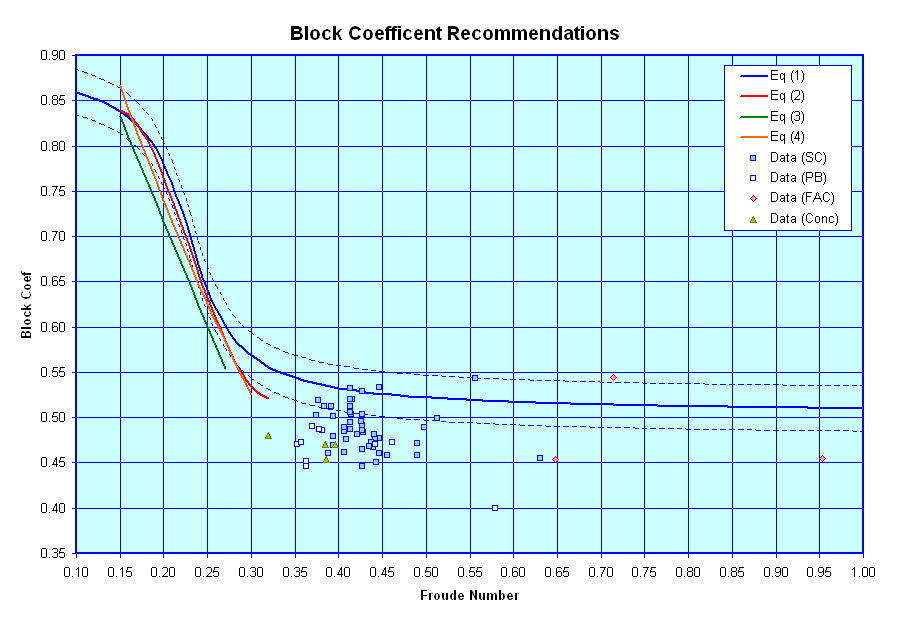
As noted on the Terminology page, a vessel's Block Coefficient is a general measure of how full its hullform is. In general for conventional displacement hulls, the slower a ship is intended to go the fuller its hullform can be. At higher speeds, however, a decrease in Block Coefficient is desirable to keep power requirements from becoming excessive. At the higher end of the speed range of conventional displacement hulls though, the benefits of further reduction in Block Coefficient tends to taper off.Within general Naval Architecture literature there are many rules of thumb for estimating recommended Block Coefficient versus the vessel's design Froude Number (or Speed/Length Ratio). Several of these recommendations are plotted in the graph below, along with a limited amount of data points for some post WWII naval designs.
In this graph:
- The Blue line represents a curve fit
recommended by Towsin in a paper by Watson & Gilfillan [Reference
6], where;
- Cb = 0.70 + 1/8 atan ((23-100*Fn)/4), and
- the dashed lines above and below this cureve represent a band of +/- 0.025
- The Red line represents a curve
recommended by Schneekluth & Bertram [Reference 7], where;
- Cb = -4.22 + 27.8*sqrt(Fn) - 39.1*Fn + 46.6*Fn^3
- The Green line represents a curve fit
recommended by Telfer for the Series 60 sysematic series of
single-screw merchant type hullforms [Reference 8], where;
- Cb = 1.18 - 0.69*Vk/sqrtL
- The Orange line represents a curve
recommended by Alexander [Reference 9], where;
- Cb = K - 0.5*Vk/sqrt(L), and
- K = 1.33 - 0.54*V/sqrt(L) + 0.24*(Vk/sqrt(L))^2
As can be seen in this figure, based on the data points shown, typical design Froude Numbers for modern naval surface combatants appear to be > 0.35 . In general, the Blue curve is the only curve that covers this region. Typical values recommended by the Blue curve in this region range from about 0.51 to 0.55 (+/- 0.025), however the data for actual ship designs suggest that actual Block Coefficients may range as low as about 0.45. As such, users may wish to enter this data themselves.
Midships Area Coefficient
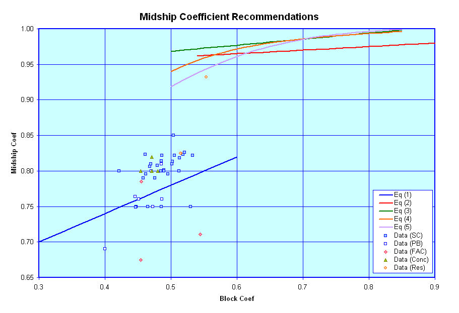
Next, here is a graph showing rules of thumb for estimating recommended Midships Coefficient versus the vessel block coefficient, along with a limited amount of data points for some post WWII naval designs.As shown in this figure, there are two general sets of curves provided. In general, as discussed on the Terminology page the midship section of a vessel may be flat bottomed, with a curved radius at its bilges, or it may have a similar shape, but with a small amount of deadrise, resulting in a slightly less full shape, or it may have a similar shape, but with a higher degree of deadrise, resuling in an even less full shape. The curve for Equation (1), which spans from a Block Coefficient from 0.3 to 0.6 represents a recommendation for a vessel's midship section with a high degree of assumed deadrise. The curve for Equation (2) represents a r ecommendation for a vessel's midship section with a low degree of assumed deadrise and Equations (3) represents a recommendation for a vessel's midship section assuming that the section is flat bottomed, with no rise of floor (deadrise). Additionally, I believe that Equations (4) and (5) represent vessel's either with no deadrise or only a very small amount.
In this graph:
- The Blue line represents a curve fit
recommended in the book Practical Ship Design by D.G.M. Watson
[Reference 10] for vessels with high deadrise, where;
- Cm = 0.40 * Cb + 0.58,
- The Red line represents a curve from
the same book for vessels with a low degree of deadrise, where;
- Cm = 0.05 * Cb + 0.935
- The Green line represents a curve fit
recommended by Benford based on the Series 60 sysematic series of
single-screw merchant type hullforms [Reference 9], where;
- Cm = 0.977 + 0.085 * (Cb - 0.60)
- The Orange line represents a curve
recommended by Kerlen [Reference 9], where;
- Cm = 1.006 - 0.0056 * Cb ^ -3.56,
- The Purple line represents a curve
based on an HSVA series of vessels [Reference 9], where;
- Cm = ( 1 + ( 1 - Cb ) ^ 3.5 ) ^ -1
Prismatic Coefficient
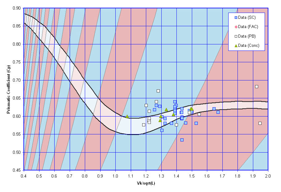
The next graph gives some guidance on Prismatic Coefficient, based on data provided in Hydrodynamics in Ship Design by H. Saunders [Reference 11] and some additional data in Principles of Naval Architecture [Reference 12] and the paper "XXXXX" by YYY [Reference 13]. The graph shows a recommended design lane (in White) for a vessel's Prismatic Coefficient based on its Speed/Length number, overlayed upon a map of theorectical humps and hollows in its resistance curve. The theorectical humps in a vessel's resistance curve are predicted to occur in the areas shaded Light Red on the graph, and the theorectical hollows are predicted to occur in the areas shaded Light Blue.
Because the wave patterns that a vessel develop while underway are dependent on the vessel's length, speed, and fullness, at different speeds a vessel may end up with its stern resting either at a peak or trough of the developed wave pattern. According to a theory outlined in the book by Saunders, when the speed of a vessel is such that the wave train it develops will result in the vessel's stern falling into a trough in the waves, the vessel will have a relative hump in its resistance curve. If the speed of the vessel is such that the wave pattern developed results in a peak at its stern, then the vessel will be closer to even trim and overall it will have a relative hollow in its resistance curve.
As shown in this graph, for the vessels that data is currently available most, though not all of them, fall into a blue shaded region of the graph and most fall at least relatively close to the suggested desing lane. Because a vessel's Prismatic Coefficient is equal to its Block Coefficient divided by its Midships Coefficient, then if the Prismatic Coefficient of a proposed design falls too far out of the proposed design lane, users may wish to try adjusting the Block Coefficient and Midships Coefficients they have chosen for the design in order to adjust the resultant Prismatic Coefficient f or the vessel. If a vessel's design speed length ratio is found to result in it falling into an area where it will be operating on a hump in its resistance curve, users can try and either;
- adjust the design's Prismatic Coefficient, which may provide small adjusts to where the design falls with respect to the humps and hollows, or
- reconsider the selected length and/or design speed, such that the proposed design speed/length ratio no longer falls on a hump, or
- the users may just decide to accept the current dimension of the design and accept that at design speed their vessel may be operating at a penalty with regards to total installed power required.
Displacement Length Ratio
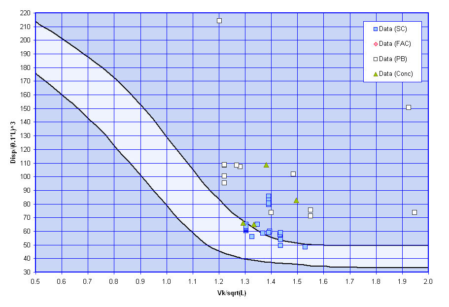
The next graph shows similar guidance on a vessel's Displacement Length Ratio, also based on data provided by Saunders [Reference 11] and some additional data in Principles of Naval Architecture [Reference 12]. The graph shows a recommended design lane for a vessel's Displacement Length Ratio (the lighter shaded section between the two black curves) for good resistance characteristics in calm water based on its Speed/Length ratio. As shown in this graph, for the vessels for which data is available some of them fall within the upper recommended bound of the Displacement Length Ratio but others fall a fair amount above this design lane. This may reflect that for modern vessels considerations other than just good calm water resistance characteristics may be driving their overall dimensions and displacement.
Waterplane Area Coeffient
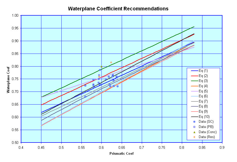
This next curve shows guidance on Waterplane Coefficient versus Prismatic Coefficient. As shown in this graph, there are numerous different curves found in literature relating Waterplane Coefficient to Prismatic Coefficient and available data on modern warships suggests that typical values of Waterplane Coefficient can fall anywhere amoung these curves with Equation (3) kind of representing an upper bound, and Equations (4) or (9) representing a lower bound, with Equation (10) coming close to an average value.
In this graph:
- The Blue line represents a curve fit
recommended for conventional hulls, where;
- Cwp = 0.73 * Cp + 0.29,
- The Red line represents a curve fit
recommended for lengthened high-speed hulls, where;
- Cwp = 0.73 * Cp + 0.32
- The Green line represents a curve fit
recommended for vessels that are to have good seakeeping, where;
- Cwp = 0.73 * Cp + 0.35
- The Orange line represents a curve
based on the Series 60 family of single-screw merchant type hullforms,
where;
- Cwp = 0.180 + 0.860 * Cp,
- The Purple line represents a curve
fit from a paper by Eames on the "Concept Exploration of Small Warship
Designs" (check title) for small transom
sterned warships, where;
- Cwp = 0.444 + 0.520 * Cp
- The Light Blue line represents a
curve fit recommended for single-screw cruiser stern hullforms, where;
- Cwp = 0.175 + 0.875 * Cp,
- The Gray line represents a curve fit
recommended for single-screw cruiser stern hullforms;
- Cwp = 0.262 + 0.760 * Cp,
- The Blue Gray line represents a curve
fit from the book "Ship Design for Economy and Efficiency" by
Schneekluth, where;
- Cwp = Cp ^ 2/3,
- The Light Orange line represents a
curve based on U-Form (need to define)
hulls, where;
- Cwp = 0.95 * Cp + 0.17 * ( 1 - Cp ) ^ ( 1 / 3 ),
- The source of the Black line is currently unknown,
where;
- Cwp = 0.23667 + 0.8333 * Cp
Half Entrance Angle
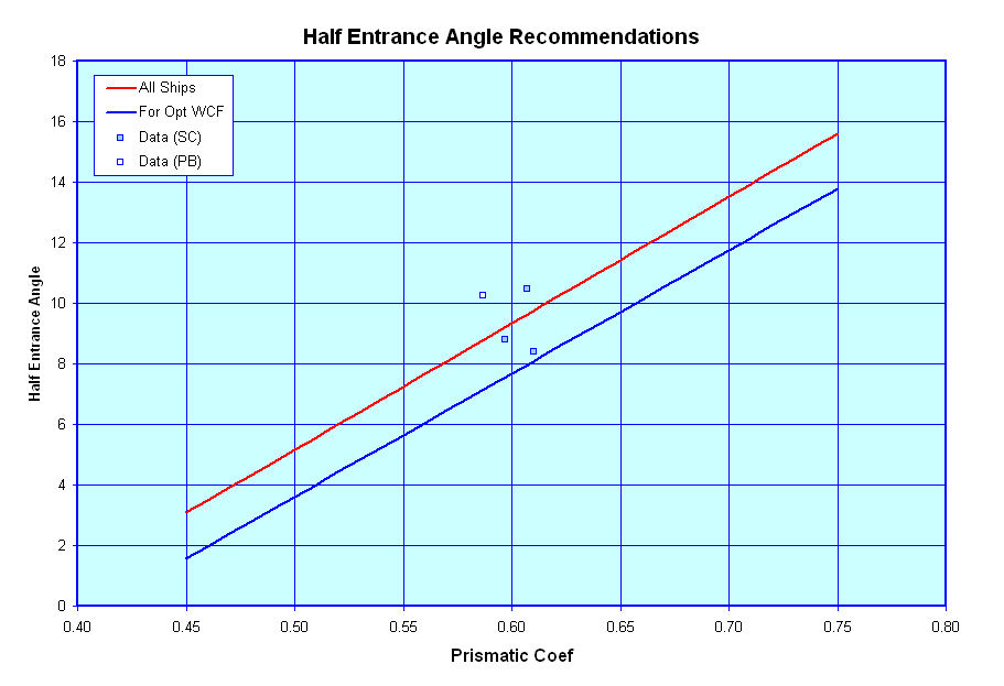
The next curve shows some recommendations for a vessel's Half Entrance Angle versus its Prismatic Coefficient. Unfortunately I only have limited data on typical Half Entrance Angles for modern naval vessels, and have not yet had a chance to review and plot them. The two curves shown though come from a paper by Sui Fung (confirm this and get title) on modern naval ship design and should be very applicable for use here. The Red Curve represented a fit through all the vessels reviewed in the referenced paper while the Blue Curve represented a fit through those vessels that were found to have very good resistance characteristics.
Longitudinal Center of Buoyancy Location
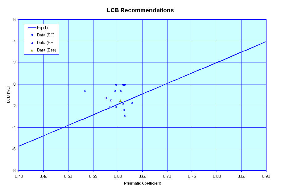
The next curve shows a recommendation for the location of a vessel's Longitudinal Center of Buoyance/LBP versus its Prismatic Coefficient. Here too I only have limited data for modern naval vessels, but I have plotted what I have and the curve of recommended values appears reasonable, based on this very limited data. The curve is attributed to Schneekluth and Bertram and comes from the book "Ship Design for Economy and Efficiency" (Ref X).
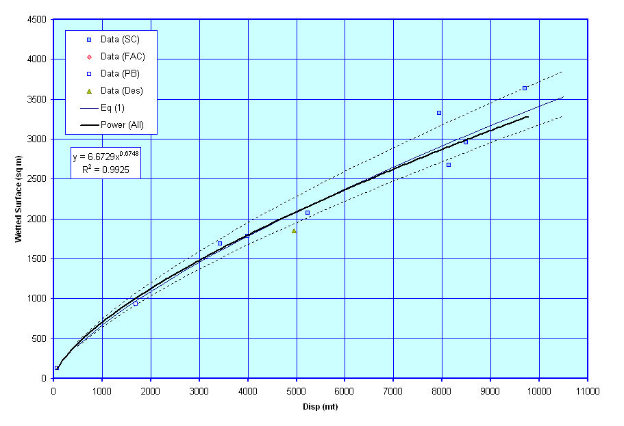
Wetted Surface Area
The next curve shows an estimate of Wetted Surface versus Displacement. It is based on an equation from Holtrop & Mennen which takes into account Midships Coefficient, Block Coefficient, Waterplane Coefficient, Length, Beam and Draft, as well as Bulbous Bow Transverse Area. For now I have assumed that bulbous bow area is zero, but for the other terms, I made use of some of the curves relating length, beam, draft, displacement, and the various hullform coefficients, discussed within this website, to come up with a notional curve of Wetted Surface verses displacement, as shown in the graph. I then investigated varying some of the terms by a small amount to develop the dashed line curves which kind of represent a notional upper and lower bound of how the wetted surface may vary from the mean line estimate. Finally, I plotted the data for the vessels I had wetted surface information on and fitted a curve through them. As can be seen in the graph, this curve fit (shown as a Thick Black line) provides very nearly the same estimate as the mean line curve based on the Holtrop & Mennen equation. In general I believe that estimating wetted surface by either means would be acceptable for this level of design.
For reference the Holtrop & Mennen equation is;
WS = L * ( B + 2 * T ) * Cm ^ ( 0.5 ) * ( 0.453 + 0.4425 * Cb - 0.2862 * Cm + 0.003467 * B/T + 0.3696 * Cw )+ 19.65 * ABT/Cb
Where ABT = the transverse area of the bulbous bow (which for now I have assumed to be zero)
The range of validity of the Holtrop & Mennen equation is listed as
- 0.55 <= Cp <=0.85
- 3.90 <= L/B <=14.9
- 2.10 <= B/T <=4.00
I have found several other equations relating Wetted Surface to other hullform parameters but have not yet tried plotting them. For reference these include;
- WS = L * ( 1.7 * T + B * Cb ), which is attributed to Denny & Mumford
- WS = 1.7 * L * T + Vol / T, which is described as a revised Denny & Mumford equation
- WS = Vol ^ ( 2/3 ) * ( 3.3 + L / ( 2.09 * Vol ^ ( 1/3 ))), which is attributed to Haslar
- WS = Vol ^ ( 2/3 ) * ( 3.4 + L / ( 2 * Vol ^ ( 1/3 ))), which is attributed to Froude
- WS = ( -0.906385E-5 * (Displ / ( L /100 ) ^ 3) ^ 2 + 0.954632E-2 * ( Displ / ( L / 100 ) ^ 3 ) + 0.776457 ) * L ^ 2 / 10, which is attributed to Baier & Bragg
- WS = C * ( L * Displ ) ^ ( 0.5 ), which is attributed to Taylor
- WS = C / 5.916 * ( L *
Vol ) ^ ( 0.5 ), which is described as a revised Taylor equation
- where C is defined as .... (need to look up)
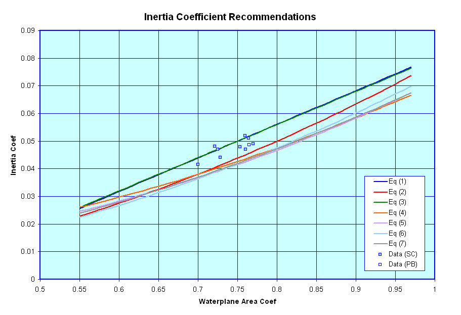
Waterplane Inertia Coeffient
This next curve shows a plot of recommended Waterplane Inertia Coefficients versus Waterplane Area Coefficient. Based on the limited data available it appears that Equations (1) and (3) give the best approximations for modern naval vessels.
In this graph:
- The Blue line represents a curve fit
attributed to D'Arcangelo, where;
- Cit = 0.1216 * Cwp - 0.0410,
- The Red line represents a curve fit
attributed to Eames for vessels with small transom, where;
- Cit = 0.0727 * Cwp ^ 2 + 0.0106 * Cwp - 0.003
- The Green line represents a curve fit
attributed to Murray (+4%), where;
- Cit = 0.04 * ( 3 * Cwp - 1 )
- The Orange line represents a curve
fit attributed to Normand, where;
- Cit = ( 0.096 + 0.89 * Cwp ^ 2 ) / 12
- The Purple line represents a curve
fit attributed to Bauer, where;
- Cit = ( 0.0372 * ( 2 * Cwp + 1 ) ^ 3 ) / 12
- The Light Blue line represents a
curve fit attributed to McGlochrie (+4%), where;
- Cit = 1.04 * Cwp ^ 2 / 12 ,
- The Gray line represents a curve fit
attributed to Dudszus & Danckwardt, where;
- Cit = ( 0.13 * Cwp + 0.87 * Cwp ^ 2 ) / 12,
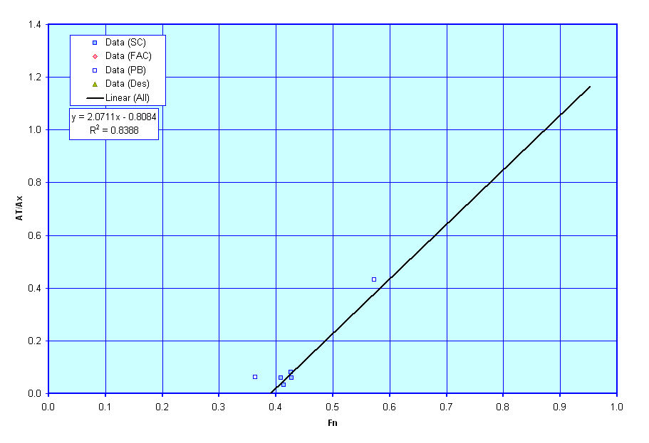
Transom Parameters
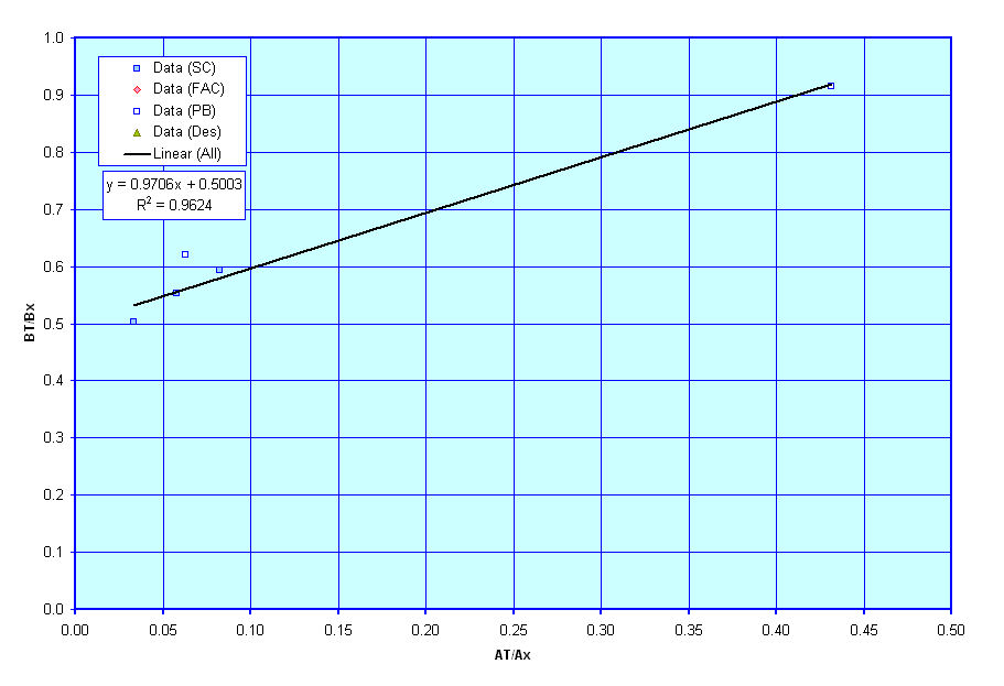
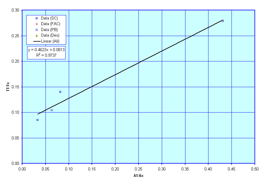
These next three curves show plots of suggested transom configuration parameters. Unlike most of the other data on this sheet which include recommendations based on equations found in general naval architectural literature, these next three graphs are currently based solely on curve fits I have tried to make through data that I have on existing ships. As such, the curves are a little rough, but are the best that I have to go on for now. As I collect and review more data I hope to update and revise these graphs.
The first graph shows a rough suggestion of Transom Area (as a % of Midships Section Area) versus the vessel's Froude Number. The second graph shows Transom Beam (as a % of vessel Beam) versus Transom Area Ratio, and the last graph shows Transom Beam (as a % of vessel Draft) versus Transom Area Ratio. These ratios are required for use in some of the resistance estimation techniques I am considering for use and thus I have put these figures together to assist users in deciding on what appropriate values of Transom Area, Beam, and Draft might be for their designs, though these are only suggestions, and users are free to select any values that they wish for these terms. Theses curves are only provided to give input on what might be reasonable estimates.
General Propeller Characteristics
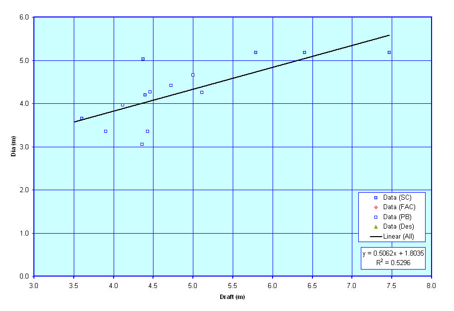
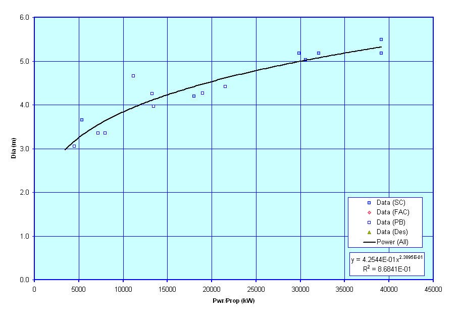
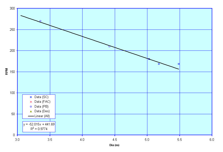
These next three curves show plots of suggested values for propeller diameter and rpm based on known data for similar vessels. Similar to the transom geometry graphs above these next three graphs are currently based solely on curve fits I have tried to make through data that I have on existing ships. As such, the curves are a little rough, but are the best that I have to go on for now. As I collect and review more data I hope to update and revise these graphs.
The first graph shows a rough suggestion of Propeller Diameter versus the vessel's Draft. The second graph shows an alternate suggestion for Propeller Diameter versus the power to be transmitted by that prop, and the last graph shows a plot of Propeller RPM vs Propeller Diameter. These values are required for use in the powering estimation techniques I am considering for use and thus I have put these figures together to assist users in deciding on what appropriate values of Propeller Diameter and RPM might be for their designs, though these are only suggestions, and users are free to select any values that they wish for these terms. They curves are only provided to give input on what might be reasonable estimates.
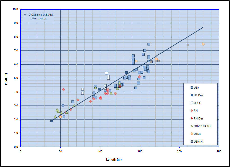
Draft
Finally, these last curve show plot of a vessel's Draft versus Length, to help the ser assess whether the resultant calculated Draft of the vessel is within the range of typical Drafts for similar vessels.