RADM DW Taylor's Mathematical Lines

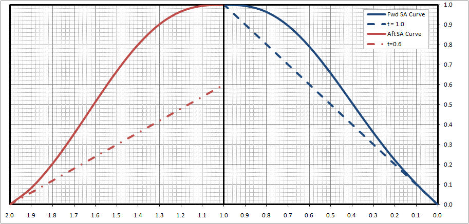
As long ago as the early 20th Century Rear Admiral David W. Taylor (USN) proposed a methodology where a ship's underwater hullform could be defined through a set of mathematical equations.   Specifically, RADM Taylor proposed that a ship's sectional area curve could be broken into segments, including the fore section, the aft section, and a mid section (if the ship has any parallel midbody).  In this scheme the fore and aft sections of the curve are approximated by fifth order polynomials, of the form:

y = tx + a x^2 + b x^3 + cx^4 + dx^5

If you non-dimensionalize the curves, where both x and y range from 0 to 1, such that;

• y = the ordinate of the sectional area curve at any atation along its length (as expressed as a fraction of the maximum)
• x = the distance along the curve.  For a ship with no parallel middle body, and an equal length fore and aft section, x = 1 would be equivalent to 1/2 the ship's Lpp
• t = the slope of the curve at its origin (numerically equal to the intercept of the tangent of the origin on the maximum ordinate (eg x = 1), see figure below

For the forward section of the sectional area curve, if we define; 

• x = 0 as the forward point of the curve 

• x = 1 as the widest point of the ship's sectional area curve

Then, if the ship does not have a bulbous bow

• @ x = 0, y = 0

• @ x = 1, y = 1

• @ x =1, y' = 0 (where y' = the 1st derivative of the curve)

       Therefor

t + 2a + 3b + 4c + 5d = 0

• @ x = 1, y" = a1 (where y" = the 2nd derivative of the curve)

y" = 2a + 6bx + 12cx^2 + 20dx^3

       Therefor

2a + 6b + 12c + 20d = a1

• the area under the curve (as defined by S y dx) = Cpf

        where,

Cpf = S (1/2 t x^2 + 1/3 ax^3 + 1/4 bx^4 + 1/5 cx^5 + 1/6 dx^6)

Cpf = 1/2 t + 1/3 a + 1/4 b + 1/5 c + 1/6 d

Then, you end up with 5 equations and 5 unknowns.  As such, it is fairly easy to solve for the coefficients, as shown below.  Specifically;

• a = 60 Cpf - 6t -30 -1/2 a1
• b = -180 Cpf + 12t +100 +2a1
• c = 180 Cpf - 10t - 105 - 5/2 a1
• d = -60 Cpf + 3t +36 + a1

The aft section of the sectional area curve can be handled similarly, as can the fore and aft ends of the design waterline.  For the aft end of the Sectional Area curve, you just need to substitute Cpa for Cpf and use an appropriate value of t to give you the shape that you wish for this section.  Similarly the value of a1 should be the negative of the value of a1 from the fore section to ensure continuity.  Typically in many/most cases a1 can often be assumed to be 0 for both segments.  For the Design Waterline, you should substitute either Cwl(fwd) or Cwl(aft) for Cpf and either the 1/2 entrance angle or the 1/2 exit angle for t, depending on which end of the waterline that you are interested in.

For the underwater hull sections RADM Taylorfound that a single equation did not appear to be suitable for all possible sections so;

• for sections with a sectional area less than about 0.75 he proposed a 4th order parabola

y = l x + ax^2 + bx^3 + cx^4

• for sections with a sectional area greater than about 0.667 he proposed a hyperbolic equation

• for sections in between 0.667 and 0.75, it was noedthat either equation gave reasonably similar shapes, as such he recommended using a sectional area of about 0.72 as the dividing point to determine which curve to use

By doing similar mathematical manipulations as above (bearing in mind that the coefficients a, b, c, and d here are not the same as those above) you can solve for the coefficients in terms of other known values.

Specifically, if;

• y = the half-breadth at any waterline as a fraction of the value at the design waterline (ie y = 1 @ x = 1)
• x = the distance above the keel as a fraction of draft (ie x = 1 @ the design waterline)
• m = the local sectional area of the section in question
• l = the recipricol of the deadrise angle for the section
• f = the flare angle for the section

Then, for the 4th order parabola

• a = 3/2 f - 9/2 l + 30 m - 12
• b = -4 f + 6 l - 60 m + 28
• c = 5/2 f - 5/2 l + 30 m + 15

And, for the hyperbola

• a = f - c ( 1 - f )
• b = ( 1 - f ) * ( 1 + c )^2
• d = ( 1 - f ) * ( 1 + c ) ^2 * c

It is harder to solve for c but since S y dx = m

Then,

m = a / 2 + b - d * loge ( ( 1 + c ) / c )

Or substituting a, b, & d from above

m = f / 2 + ( 1 - f ) ( 1 + c ) ^2 [ 1 - c / ( 2 * ( 1 + c ) ^ 2) - c * loge ( ( 1 + c ) / c ) ]

Using a spreadsheet like MS Excel it becomes fairly easy to set up an interpolation table, where for various values of m and f you can estimate the appropriate value of c to use.

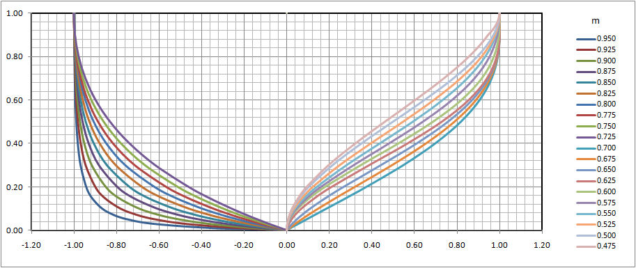
The figure below shows a set of section shapes developed using this methodology, for a section area ratio (m) ranging from 0.475 to 0.95, with  flare angle (f) of zero.

An important factor to bare in mind here, is that when using this method for drawing up a ship's rough lines, you will have to transform some data for use.  Specifically, using the polynomial equations for the Design Waterline and Sectional Area Curve can give you values for 1/2 breadth as a fraction of the ship's maximum overall 1/2 breadth, and sectional area for the station as a fraction of the ship's maximum sectional area.  To draw the actual section shape you should then transform the sectional are value that you get from the equations into full scale sectional area, and then figure out what the local sectional area value would be for the max beam and draft at that station.

The method outlined above can be very useful, but because it treats the fore and aft sections of the ship separately, it relies on inputs of hullform coefficients such as Cpf, Cpa, Cwl (fwd), Cwl(aft), LCB(fwd), LCB(aft), LCF(fwd), and LCF(aft), etc that are not commonly available for most ships.

Home