

Resistance & Powering
Resistance Estimation Method
The resistance estimation method that I am using in the spreadsheet I have developed is based on;
- a residuary resistance estimation method developed by Sui Fung and Larry Leibman for transom hulled vessels that was presented at the FAST 1995 conference.
- a frictional resistance estimation based on the ITTC 1957 curve,
- an appendage resistance estimation based on a method outlined in the US Navy's Design Data Sheet 051-1 (DDS 051-1) "Prediction of Smooth-Water Powering Performance for Surface-Displacement Ships", and
- a wind resistance and still air drag estimation based on a method attributed to RADM David W. Taylor, as described in the book "Principles of Naval Architecture".
Residuary Resistance - The residuary resistance method I mentioned above is a revision/extension to an earlier method that was published by these same authors in a Chesapeake Section of the Society of Naval Architects and Marine Engineers (SNAME) paper in 1993 and is also similar to (though slightly differently formatted from) a method presented by Sui Fung in the Transactions of SNAME in 1991. In order to keep help clarify things I will refer to the initial method from the 1991 paper as the Fung-Transom Stern Hull or F-TSH method, the method presented in the 1993 SNAME Chesapeake Section paper as the Fung & Leibamn or F&L method, and the revised method presented in at the FAST 1995 conference as the revised Fung & Leibman or F&L 2 method.
I selected the F&L 2 method for use here because it appears well suited to the modern naval surface combatant type vessels and is a little easier to use than methods like the NSMB/H&M method.
In the F&L 2 method residuary resistance is estimated based on 70 coefficients and a vessel's Displacement-Length Ratio (DLR), Transom Area Coefficient (TA), Prismatic Coefficient (Cp), Transom Width Ratio (TW), Beam to Draft Ratio (B/T), Half Entrance Angle (ie), Midship's Coefficient (Cm), and Wetted Surface Area (WSA). The coefficients used in estimating residuary resistance were developed from a multiple linear regression analysis of the residuary resistance of 739 different High-Speed Transom-Stern models in the US Navy's High-Speed Transom-Stern (HSTS) database including a total of 10,672 different resistance datapoints.
In this method;
Cr = exp{ S [ Bi P (xj Cij)]}
Where;
- X1 = Fnd
- X2 = cos (l * Fn e) * exp (a/Fn2)
- X3 = {0.034977 * [D/(L/100)3]}0.5
- X4 = AT
- X5 = Cp2
- X6 = BT
- X7 = B/T
- X8 = LN( 90 - ie )
- X9 = Cm
- D = Displacement
- l = [ a1 * Cp + a2 * D/(L/100)3]
- a = - 0.2000
- a1 = 0.7500
- a2 = 0.0350
- d = - 0.7000
- e = - 1.9300
- n = 69 (eg. the number of terms in regression model excluding the constant)
- S = the summation operator from i = 0 to i = n (eg. it means sum all these terms together)
- P = the multiplication operator from j = 0 to 9 (eg. it means multiply all these terms together)
- Bi = the regression coefficients (as summarized in the table below)
| Bi | X1 | X2 | X3 | X4 | X5 | X6 | X7 | X8 | X9 | Bi | X1 | X2 | X3 | X4 | X5 | X6 | X7 | X8 | X9 | |||
| 0 | -0.0768852 | 0 | 0 | 0 | 0 | 0 | 0 | 0 | 0 | 0 | 35 | -0.6353710 | 2 | 0 | 0 | 1 | 0 | 0 | 0 | 0 | 0 | |
| 1 | -5.3817900 | 1 | 0 | 0 | 0 | 0 | 0 | 0 | 0 | 0 | 36 | -0.2575700 | 2 | 0 | 0 | 0 | 0 | 1 | 0 | 0 | 0 | |
| 2 | -7.3172000 | 0 | 1 | 0 | 0 | 0 | 0 | 0 | 0 | 0 | 37 | -0.0217107 | 2 | 0 | 0 | 0 | 0 | 0 | 1 | 0 | 0 | |
| 3 | 4.0212100 | 0 | 0 | 1 | 0 | 0 | 0 | 0 | 0 | 0 | 38 | 0.5663620 | 1 | 2 | 0 | 0 | 0 | 0 | 0 | 0 | 0 | |
| 4 | -3.0154100 | 0 | 0 | 0 | 1 | 0 | 0 | 0 | 0 | 0 | 39 | -0.4384070 | 1 | 1 | 1 | 0 | 0 | 0 | 0 | 0 | 0 | |
| 5 | -3.3034700 | 0 | 0 | 0 | 0 | 0 | 1 | 0 | 0 | 0 | 40 | -2.1790300 | 1 | 1 | 0 | 1 | 0 | 0 | 0 | 0 | 0 | |
| 6 | -0.3560160 | 0 | 0 | 0 | 0 | 0 | 0 | 1 | 0 | 0 | 41 | -0.1157800 | 1 | 1 | 0 | 0 | 0 | 0 | 1 | 0 | 0 | |
| 7 | -0.7864200 | 0 | 0 | 0 | 0 | 0 | 0 | 0 | 1 | 0 | 42 | 0.1795660 | 1 | 0 | 2 | 0 | 0 | 0 | 0 | 0 | 0 | |
| 8 | 0.5219150 | 2 | 0 | 0 | 0 | 0 | 0 | 0 | 0 | 0 | 43 | -0.4294660 | 1 | 0 | 1 | 1 | 0 | 0 | 0 | 0 | 0 | |
| 9 | 3.6728900 | 1 | 1 | 0 | 0 | 0 | 0 | 0 | 0 | 0 | 44 | -0.2797660 | 1 | 0 | 1 | 0 | 0 | 1 | 0 | 0 | 0 | |
| 10 | -0.5265970 | 1 | 0 | 1 | 0 | 0 | 0 | 0 | 0 | 0 | 45 | 0.0317788 | 1 | 0 | 1 | 0 | 0 | 0 | 1 | 0 | 0 | |
| 11 | 3.6657800 | 1 | 0 | 0 | 1 | 0 | 0 | 0 | 0 | 0 | 46 | -0.3435530 | 1 | 0 | 1 | 0 | 0 | 0 | 0 | 0 | 1 | |
| 12 | 2.9864900 | 1 | 0 | 0 | 0 | 1 | 0 | 0 | 0 | 0 | 47 | -2.2750200 | 1 | 0 | 0 | 2 | 0 | 0 | 0 | 0 | 0 | |
| 13 | 2.9831400 | 1 | 0 | 0 | 0 | 0 | 1 | 0 | 0 | 0 | 48 | 3.6338800 | 1 | 0 | 0 | 1 | 0 | 1 | 0 | 0 | 0 | |
| 14 | 0.3224910 | 1 | 0 | 0 | 0 | 0 | 0 | 1 | 0 | 0 | 49 | -0.1088050 | 1 | 0 | 0 | 1 | 0 | 0 | 1 | 0 | 0 | |
| 15 | 1.3066300 | 1 | 0 | 0 | 0 | 0 | 0 | 0 | 0 | 1 | 50 | -2.5626000 | 1 | 0 | 0 | 0 | 1 | 1 | 0 | 0 | 0 | |
| 16 | 2.1950800 | 0 | 2 | 0 | 0 | 0 | 0 | 0 | 0 | 0 | 51 | -0.1188630 | 1 | 0 | 0 | 0 | 0 | 1 | 1 | 0 | 0 | |
| 17 | 6.3962400 | 0 | 1 | 0 | 1 | 0 | 0 | 0 | 0 | 0 | 52 | -0.1846400 | 1 | 0 | 0 | 0 | 0 | 0 | 1 | 0 | 1 | |
| 18 | 3.3582200 | 0 | 1 | 0 | 0 | 1 | 0 | 0 | 0 | 0 | 53 | -0.2616470 | 0 | 2 | 1 | 0 | 0 | 0 | 0 | 0 | 0 | |
| 19 | 0.3036790 | 0 | 1 | 0 | 0 | 0 | 0 | 1 | 0 | 0 | 54 | -3.8195800 | 0 | 2 | 0 | 0 | 1 | 0 | 0 | 0 | 0 | |
| 20 | -1.4792000 | 0 | 1 | 0 | 0 | 0 | 0 | 0 | 0 | 1 | 55 | 0.1225660 | 0 | 1 | 2 | 0 | 0 | 0 | 0 | 0 | 0 | |
| 21 | -0.9375770 | 0 | 0 | 2 | 0 | 0 | 0 | 0 | 0 | 0 | 56 | -0.2800950 | 0 | 1 | 1 | 0 | 0 | 1 | 0 | 0 | 0 | |
| 22 | 0.8657370 | 0 | 0 | 1 | 1 | 0 | 0 | 0 | 0 | 0 | 57 | -0.0338132 | 0 | 1 | 1 | 0 | 0 | 0 | 1 | 0 | 0 | |
| 23 | -0.5543990 | 0 | 0 | 1 | 0 | 1 | 0 | 0 | 0 | 0 | 58 | 0.3287260 | 0 | 1 | 1 | 0 | 0 | 0 | 0 | 0 | 1 | |
| 24 | 0.5885840 | 0 | 0 | 1 | 0 | 0 | 1 | 0 | 0 | 0 | 59 | -5.6044500 | 0 | 1 | 0 | 1 | 1 | 0 | 0 | 0 | 0 | |
| 25 | -0.1395060 | 0 | 0 | 1 | 0 | 0 | 0 | 1 | 0 | 0 | 60 | 0.4034580 | 0 | 1 | 0 | 0 | 0 | 2 | 0 | 0 | 0 | |
| 26 | 0.6936350 | 0 | 0 | 1 | 0 | 0 | 0 | 0 | 0 | 1 | 61 | 0.7806980 | 0 | 1 | 0 | 0 | 0 | 1 | 0 | 0 | 1 | |
| 27 | -7.4962600 | 0 | 0 | 0 | 1 | 0 | 1 | 0 | 0 | 0 | 62 | 0.3615190 | 0 | 0 | 2 | 1 | 0 | 0 | 0 | 0 | 0 | |
| 28 | -0.6192280 | 0 | 0 | 0 | 1 | 0 | 0 | 1 | 0 | 0 | 63 | 0.0332259 | 0 | 0 | 2 | 0 | 0 | 0 | 1 | 0 | 0 | |
| 29 | 2.0395900 | 0 | 0 | 0 | 0 | 1 | 1 | 0 | 0 | 0 | 64 | -0.9738470 | 0 | 0 | 1 | 2 | 0 | 0 | 0 | 0 | 0 | |
| 30 | 0.3454600 | 0 | 0 | 0 | 0 | 1 | 0 | 1 | 0 | 0 | 65 | -0.1611350 | 0 | 0 | 1 | 1 | 0 | 0 | 1 | 0 | 0 | |
| 31 | -5.4932300 | 0 | 0 | 0 | 0 | 1 | 0 | 0 | 0 | 1 | 66 | 4.1889600 | 0 | 0 | 0 | 2 | 1 | 0 | 0 | 0 | 0 | |
| 32 | 0.2514840 | 0 | 0 | 0 | 0 | 0 | 1 | 1 | 0 | 0 | 67 | 0.7622500 | 0 | 0 | 0 | 2 | 0 | 0 | 1 | 0 | 0 | |
| 33 | -0.9467220 | 0 | 0 | 0 | 0 | 0 | 1 | 0 | 0 | 1 | 68 | 1.5920600 | 0 | 0 | 0 | 1 | 0 | 2 | 0 | 0 | 0 | |
| 34 | 0.6660340 | 0 | 0 | 0 | 0 | 0 | 0 | 0 | 0 | 2 | 69 | 0.7761980 | 0 | 0 | 0 | 1 | 0 | 0 | 1 | 0 | 1 |
The range of applicability for this method is;
- Fn between 0.15 & 0.90
- DLR between 16.239 & 359.180
- LCB between 0.481 & 0.591
- ie between 2.600 & 31.730
- L/B between 2.520 & 17.935
- B/T between 1.696 & 10.204
- Cp between 0.526 & 0.774
- Cm between 0.556 & 0.994
- Cwp between 0.662 & 0.841
- TA between 0.00 & 0.740
- TB between 0.000 & 1.000
- TT between 0.000 & 0.770
- Cws (Wetted Surface Coefficient) between 14.324 & 23.673
Frictional Resistance - The fricitional resistance method I mentioned above is the ITTC 1957 method as described on the Background page where;
Cf = 0.075/(log10 (Rn) - 2)2Where Rn = Reynold's number and is is defined as;
Rn = v L / n
Where;
v = the vessel's speed
L = the vessels length
n = the kinematic visosity of water
(all in consistant units)
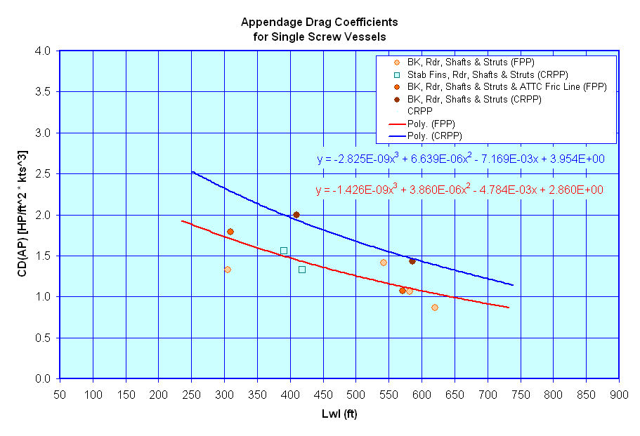
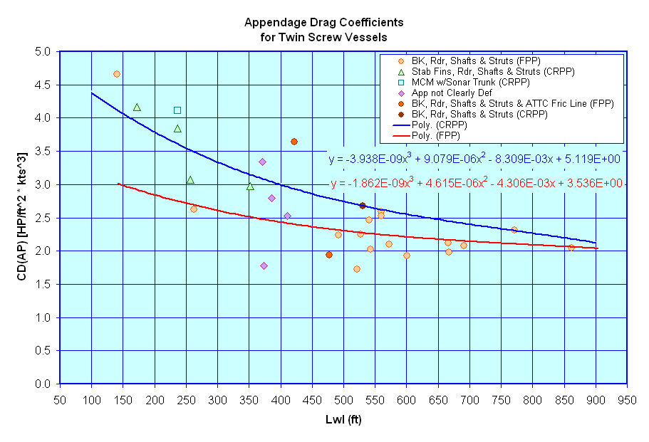
Appendage Resistance - The appendage resistance method I mentioned above is based on information provided in DDS 051-1 as shown in the two figures below.
These figures show the recommended Appendage Drag Coefficients from DDS 051-1 for both twin screw vessels and single screw vessels. [Please note that this data is in semi-imperial units (ie they are not in metric or non-dimensional units) and as such care must be taken when using them to ensure the units come out correctly.]
Wind Resistance & Still Air Drag - As a ship moves through the water it encounters resistance to this motion not only from the water it is moving through, but also the air that the portion of the ship above the waterline comes in contact with. For early stage design, I believe that we are most interested in either
- only the still air drag generated solely from the ship's forward motion (condition 1), or
- the still air drag generated from the ship's forward motion plus a certain amount of head wind acting on the front of the vessel (condition 2)
As noted on the Background sheet, there is a simplified equation that was proposed by RADM D.W. Taylor in 1943 very suitable for early stage design. In it;
Raa = 0.783 * ½ * B2 VR2
Where;
- Raa = The total added air resistance
- B = the Beam of the ship (in meters)
- VR = the apparent relative wind velocity (for condition 1 this would be equal to the forward speed of the ship, but in condition 2 this would include both the speed of the ship and any additional head wind) (in meters per second)
I have selected this version of the equation for use as it doesn't require an estimate of frontal area, which may not be fully known in early stage design. In the future I may consider updating this section however, to ensure that the resistance of vessels with non-traditional deckhouse sizes are adequately addressed.
Total Resistance Estimate Examples - The figures below show a comparison of published resistance data for the FFG 7, DD 963, a DDG 51 class vessel, a CG 47 class vessel, and the resistance for these vessels as estimated using the above methods. For reference I have also included an estimate of the resistance for these vessels based on the more complex Holtrop & Mennen/NSMB method.
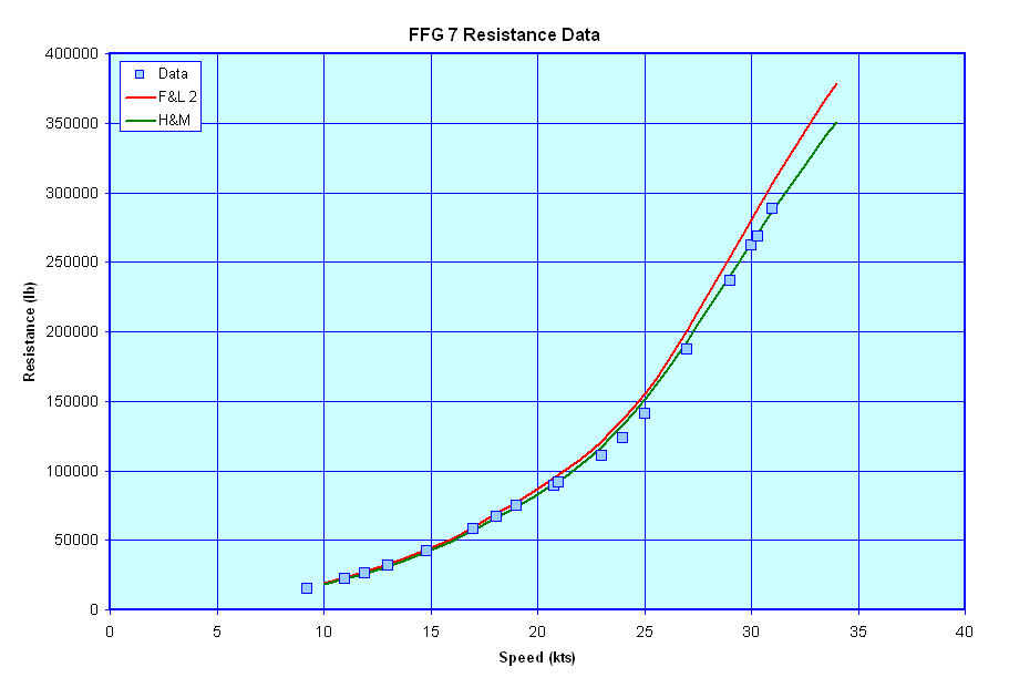
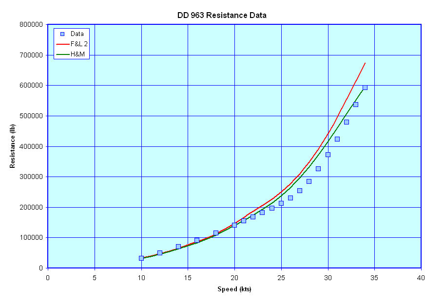
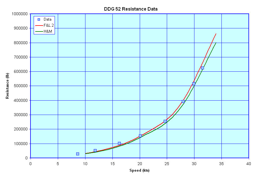
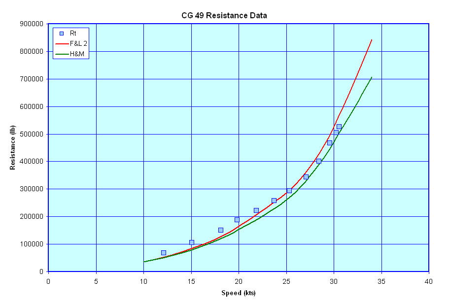
As can be seen from these figures both the F&L 2 and H&M methods give relatively good approximations of the resistance for these vessels, with the F&L 2 method being perhaps just a bit more conservative. One other thing of note is that both methods appear to over estimate the resistance of the DD 963 class vessel whereas the resistance estimates for the CG 47 class vessel, which shares a common hullform with the DD 963 class ships, are more in line with the CG 47 class vessels reported resistance. As such, I want to go back a review the data for those two vessels to ensure that all the calcs have been done correctly and the correct displacements and drafts (etc) for both vessels have been correctly used for each vessel.